Regression is a technique used to predict a dependent variable given one or more independent variables. Linear regression as the name implies is specifically used when there is a linear relationship between the dependent and independent variable. The relationship between the variables can be described using an equation that is referred to as a model or the line of best fit (LOBF). The general form is:
![]()
This is just the equation of a line, ![]() , but the notation used in statistics is different. Similarly to the equation for a line,
, but the notation used in statistics is different. Similarly to the equation for a line, ![]() is the y-intercept and
is the y-intercept and ![]() is the slope.
is the slope. ![]() is referred to as the dependent variable or response and
is referred to as the dependent variable or response and ![]() is the independent variable or predictor.
is the independent variable or predictor.
Topics Covered
Common Questions
Correlation
The Model
Interpretation
Hypothesis Test and Confidence Interval
Residual
Common Questions
When covering the chapter of linear regression, the following kinds of questions are most commonly asked:
- Finding and interpreting the correlation,

- Write the theoretical and estimated model
- Read software output (JMP, Excel)
- Interpret the slope (
 ) and y-intercept (
 )
) - Interpret the coefficient of determination,

- Conduct a hypothesis test for

- Create a confidence interval for

- Calculate a residual
This is not a definitive list. Ask your professor or instructor for other types of questions that will be on the exam.
top
Correlation
Correlation measures the linear relationship between two variables. The sample correlation is represented as ![]() , while the population correlation is represented as
, while the population correlation is represented as ![]() (Greek letter rho). It is important to keep in mind that
(Greek letter rho). It is important to keep in mind that ![]() can only be between 1 and -1.
can only be between 1 and -1.
When ![]() , the variables will have the following characteristics:
, the variables will have the following characteristics:
- The variables are positively correlated
- As one increases the other variable increases
- The variables will be upward sloping
When ![]() , the following characteristics apply:
, the following characteristics apply:
- The variables are negatively correlated
- When one increases the other variable decreases
- The variables will be downward sloping
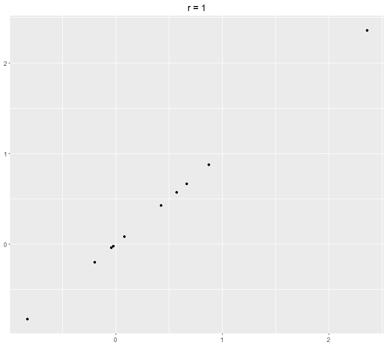
When ![]() , the variables have a perfect positive linear relationship. This means that when the variables are plotted on a scatter plot, they will form a straight upward sloping line. When
, the variables have a perfect positive linear relationship. This means that when the variables are plotted on a scatter plot, they will form a straight upward sloping line. When ![]() , the variables have a perfect negative linear relationship. When the variables are plotted on a scatter plot, they will form a straight downward sloping line. When
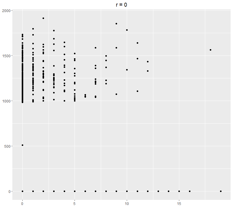
, the variables have a perfect negative linear relationship. When the variables are plotted on a scatter plot, they will form a straight downward sloping line. When ![]() , there is no linear relationship between the variables. When they are plotted, it will look like either a horizontal or vertical line.
, there is no linear relationship between the variables. When they are plotted, it will look like either a horizontal or vertical line.
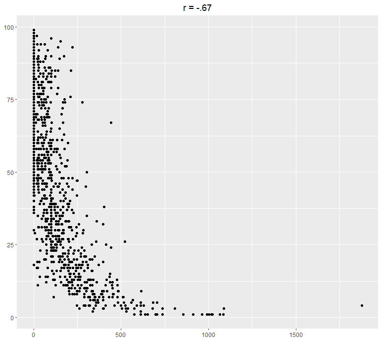
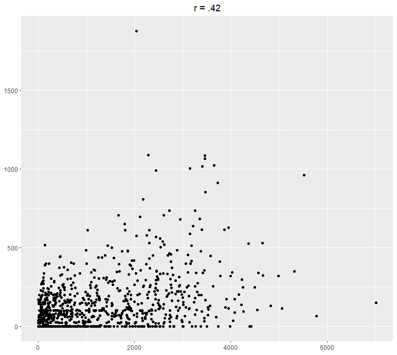
Here are some examples of two variables plotted using a scatter plot and their following correlation:
The Model
To cover the following topics, we will be using an example from the video game PlayerUnknown’s Battlegrounds (PUBG). It is a game similar to Fortnite, where 100 players are dropped in a map. The goal of the game is to eliminate all other players using a variety of weapons and be the last one standing. In this example, we will be trying to predict how much total damage a player dealt to other players given how many kills they got in a match. The first step is to write the Theoretical Model:
![]() or
or ![]()
Some important things to note when writing the theoretical model:
- Capital letters are used, such as Y, X,
 ,
, 
 : y-intercept
 : population slope
 : random error, only gets included with the theoretical model
 : the dependent or response variable
 : the independent or predictor variable
Now we can use either Excel or JMP to run the regression analysis and be able to write the Estimated Model. The following output is from Excel, but JMP output should have the same information.
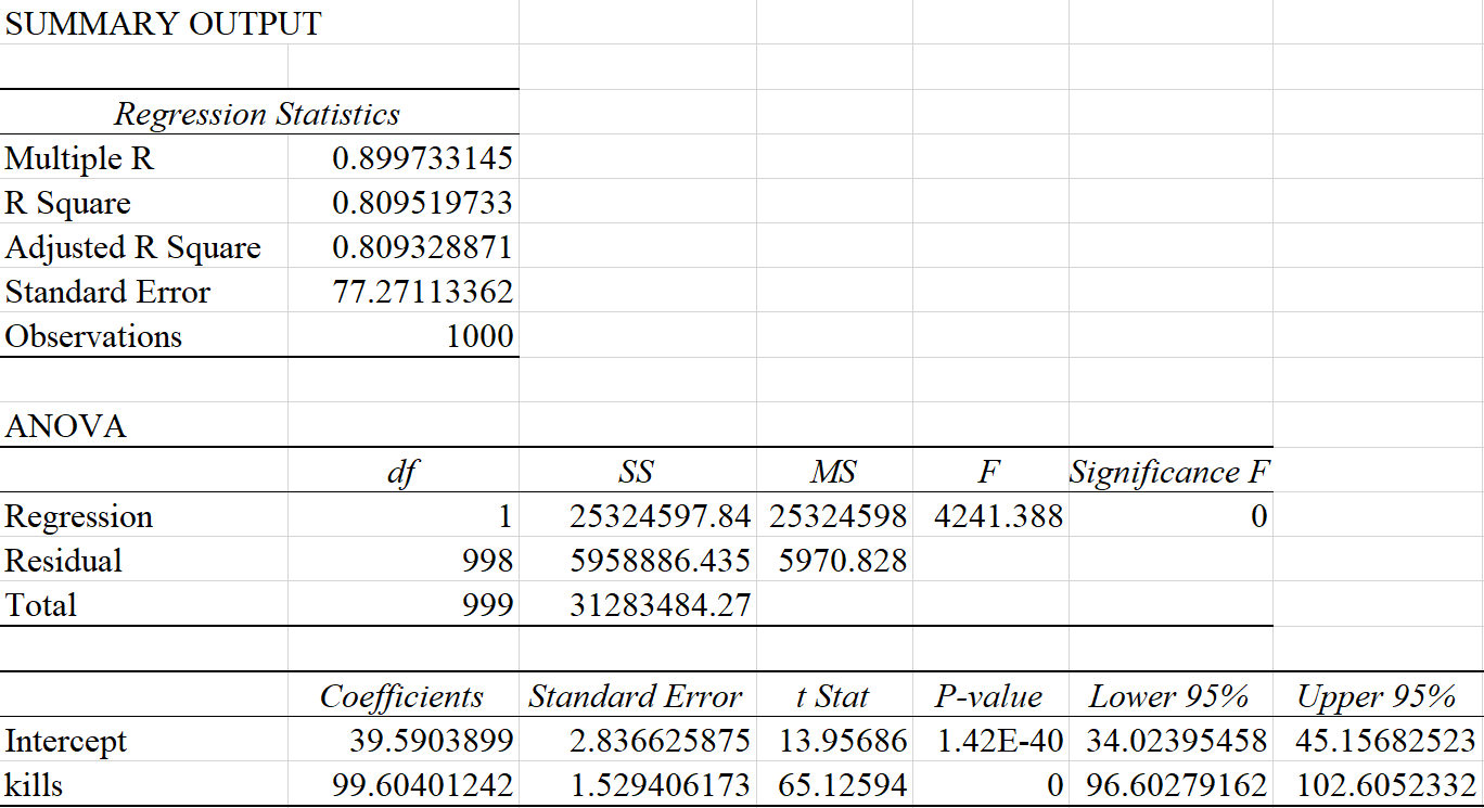 To write the estimated model we have to look at the third table, under the Coefficients column. The first row is dedicated to information about the y-intercept and the second row is dedicated to information about the slope. So our estimated model will look like this:
![]() or
or ![]()
Keep the following in mind when writing the estimated model:
- Add a hat (
 ) to the dependent variable
 - Use lower case letters, such as y,
 ,
, 
- The random error term (
 ) is not included
Interpretation
We are usually asked to interpret the slope, y-intercept, and coefficient of determination (![]() ) and in most cases in can be done in a formulaic way. The following interpretations are generalized and will have to be put in the context of the problem.
) and in most cases in can be done in a formulaic way. The following interpretations are generalized and will have to be put in the context of the problem.
- Y-intercept (
 ): When X is equal to 0, Y is equal to
- Slope (
 ): When X is increased by 1 unit, Y changes by the slope
  : the proportion of variability in the response that can be explained by the model.
- This value is found under the first table.
Example:
- Y-intercept: When a player has 0 kills, the predicted total damage dealt is 39.590.
- Slope: When a players kill count increases by 1, their predicted total damage dealt increases by 99.604.
 : 80.95% of the variability in damage dealt can be explained by the model.
Hypothesis Test and Confidence Interval
One way to determine if there is a linear relationship between two variables is by evaluating their correlation. Another way is by evaluating the slope from the model. If the population slope (![]() ) is zero, it means that there is no relationship between the variables and the predictor variable is not significant. To evaluate the slope, we can either perform a hypothesis test or a confidence interval. In either case, we should end up with the same conclusion.
) is zero, it means that there is no relationship between the variables and the predictor variable is not significant. To evaluate the slope, we can either perform a hypothesis test or a confidence interval. In either case, we should end up with the same conclusion.
Hypothesis Test
Hypothesis test for the slope will all have the same setup:
![]()
![]()
![]()
The test statistic and the corresponding P-Value can be found in the third table of our output.
Note: Sometimes they will not give the test statistic and you will have to calculate it by hand.
EX:
Our test statistics is equal to:
![]()
Since the corresponding P-Value is approximately 0, we reject the null hypothesis and conclude that ![]() differs from 0.
differs from 0.
Confidence Interval
The general formula for the CI is:
![]()
Sometimes the CI will be given to you in the summary table. If you are asked to calculate it by hand, most of the information should be given to you in the summary output. The only value that changes will be the critical value, which will depend on the confidence level. After the CI is calculated, we check if 0 is in or out of our CI. If 0 is outside the CI, we conclude that ![]() significantly differs from 0. If 0 is inside the CI, we conclude that
significantly differs from 0. If 0 is inside the CI, we conclude that ![]() does not significantly differs from 0.
does not significantly differs from 0.
EX:
To create the CI, we pull the values straight from the third table in the summary output. For a 95% CI we will approximate the critical value by using 2.
![]()
We notice that 0 is not in our CI, so we can conclude that ![]() significantly differs from 0.
significantly differs from 0.
top
Residual
A residual tells us how much our prediction was off by. We can calculate a residual for every value. If a value has a residual of 0, it means that our model predicted the response accurately. The formula is as follows:
![]()
EX:
Suppose we are asked to calculate the residual for when a player has 2 kills. In our data set, we observe that a player with 2 kills dealt a total damage of 200. The predicted value is calculated using our line of best fit.
![]()
![]()
