The Central Limit Theorem (CLT) states that the sampling distribution of the means will become a normal distribution as the sample size increases. To understand the CLT, we first have to have a good grasp of the sampling distribution. The sampling distribution arises from repeatedly sampling a statistic. This is done by getting a random sample of size n from our population and then calculating some statistic from that sample such as the mean, standard deviation, or variance. We do this over and over until we get a new data set that is now is composed of the statistic we calculated from our samples.
The distribution from the raw data will give us an idea of what are the possible values our population can take and how frequent those values appear. This distribution will have some mean and standard deviation. The sampling distribution for the means will show us the possible means we can get from getting different random samples. This sampling distribution will have a similar mean to our distribution mean, but with a different standard deviation. The standard deviation of the sampling distribution is referred to as the standard error and it is the standard deviation from our distribution divided by the square root of the sample size.
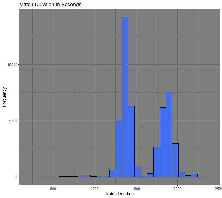
To show the CLT in action, I have provided an example using a data set from the video game PlayerUnknown’s Battlegrounds (PUBG). This is a game similar to Fortnite, where it consist of 100 players being dropped on the same map. The goal of the game is to eliminate all other players and be the last one standing. What we are focusing for this example is the duration of a match. Below you will see a distribution of the match lengths. It is bimodal since it has two peaks around 1400 and 1800 seconds. The mean is equal to 1579 and the standard deviation is 264.
The next step is to get different sampling distributions with increasing sample sizes. The following graphs consist of 500 random samples of sample size 5, 20, and 50.
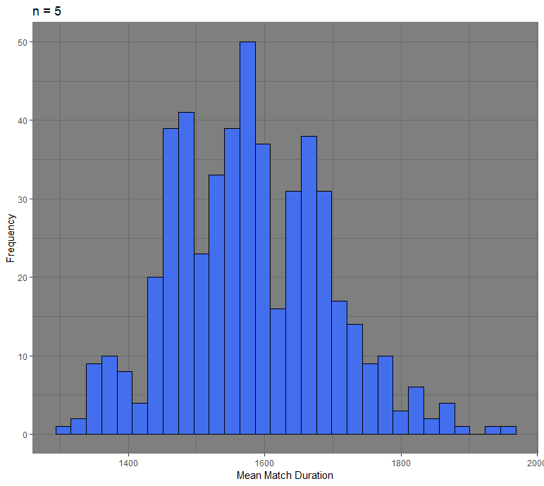
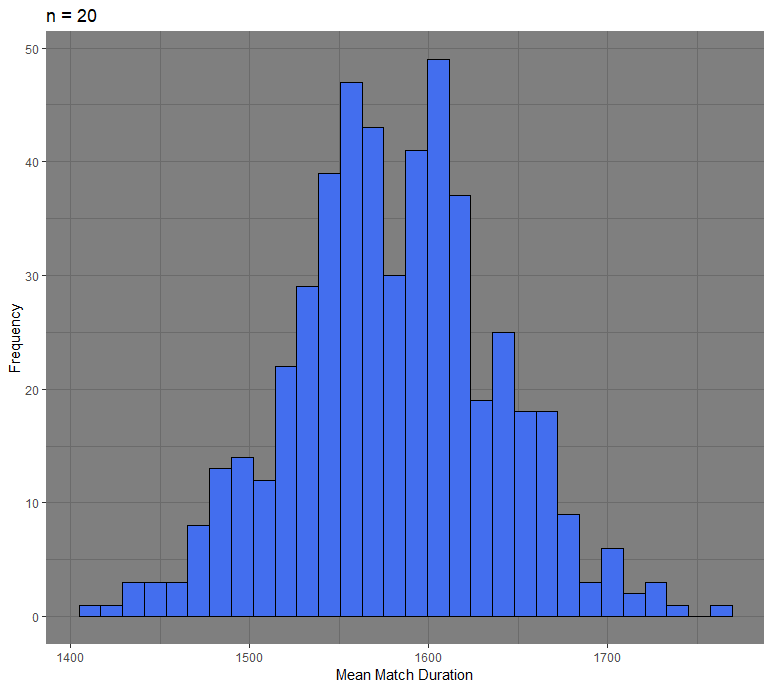
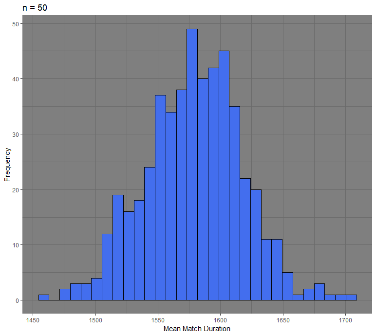
We see that as the sample size increases, the distribution becomes more normal. The sampling distribution with a sample size of 50 has a mean of 1579, similar to the average of our original distribution. The standard error is 37 and is also what we would approximately get if we were to follow the standard error formula.
The CLT is a powerful theory that allows us to perform inference for the population mean. We are able to create confidence intervals and do hypothesis testing, which rely on the normal distribution. Even though the original distribution might not be normal, the CLT assures the sampling distribution for the means will be.